|
General Notation: The Data Hierarchy - Trees, Nodes, and Models
The basic data structure of MDSplus is a self-descriptive hierarchy called a TREE. The hierarchy consists of large numbers of named NODES which make up the branches (structure) and leaves (data) of each tree. MDSplus SHOTS are trees created from a special type of tree called a MODEL, a template which contains all of the structure and setup data for an experiment or code. SHOTS are copies of the model augmented by the stored data and correspond to particular runs of an experiment or code. For a typical experiment, data from various sources are grouped in some logical manner and divided into a number of trees which each form the top level of their respective hierarchies. These trees themselves can be organized into a hierarchy with a root tree and SUBTREES as in the following figure.
In the rest of this section we shall discover how MDSplus data structures can be created and accessed. Let's start!
How to create and populate a MDSplus tree
In this first lesson we shall build a very simple MDSplus tree. A MDSPlus tree is a database which contains several types of data. A data item may be a number, a string, a signal or, more generally an expression i.e. a combination of data (possibly stored in the same tree) and operators.
Besides data, the nodes of a MDSplus tree may contain other kind of information, but we shall discuss about it in the following tutorials.
The MDSplus tree represents the core of MDSplus, and there are many ways for interacting with it. Here, we shall use two tools:
1) The Tree Command Language (TCL, not to be confused with TCL/TK) for creating and editing a tree;
2) The jTraverser tool for providing a graphical interface to the tree.
A Quick Check for some important environment variables
Before starting working with MDSplus, it is important to make sure that a few environment variables are properly set. When installed via an install shield or RPM, the variables should be ok, but in the case MDSplus is build from the source distribution, the following variables must be defined for Linux:
- LD_LIBRARY_PATH this variable is used by the Operating System to locate dynamic libraries, which are listed separated by a colon. <MDSPlusRoot>/lib must be included.
- PATH: must include directory <MDSplusRoot>/bin
- MDS_PATH must be defined as <MDSplusRoot>/tdi
- CLASSPATH must include (separated by colon) <MDSplusRoot>/java/classes/jScope.jar, <MDSplusRoot>/java/classes/jTraverser.jar, <MDSplusRoot>/java/classes/jDevices.jar, <MDSplusRoot>/java/classes/MDSobjects.jar, <MDSplusRoot>/java/classes/jDispatcher.jar
The creation of a sample tree
Before starting we need to define an environment variable which indicates to MDSplus the location of the tree. Let's call the new tree my_tree, so we need to define the environment variable my_tree_path (NOTE: you must use lowercase letters for this variable) to the directory which will contain the database (the general rule for the variable name is <tree name>_path). Make sure you have write privilege in the target directory.
On Linux (using bash) we define the environment variable as follow:
export my_tree_path = <directory>
On windows, things are a bit more complicated. These are the required steps:
1) Open the Control Panel
2) Select System
3) Select Advanced Tab
4) Select "Environment variables"
5) If adding a new variable select New
6) In "Variable name" and "Variable Value" write the the name (<tree_name>_path) and the value (the directory which will contain pulse files)
Note that on Windows, the variable is defined forever, while on Linux you need to define it for each session, therefore it is convenient to put the definition in a shell script, such as .bashrc.
Now, we shall create a tree containing three nodes:
NUM1 containing a number
NUM2 containing an array
NUM3 containing an expression
TXT containing a string
Let's do it using TCL:
1) Start TCL
TCL is started from a terminal by the command mdstcl. On Windows system TCL can also be started by selecting the TCL menu item in the MDSplus menu.
TCL provides a complete online help, just type
TCL> help
for an help overview, or
TCL> help tree commands
explaining commands for manipulating MDSplus trees
2) Create a new tree:
TCL> edit my_tree/new
3) Add node NUM1:
TCL>add node NUM1/usage=numeric
This command creates a new node named NUM. It will contain numeric data, but currently is empty.
4) Fill node NUM1:
TCL>put NUM1 "2"
This command fills node NUM1 with the number 2.
3) Add node NUM2:
TCL>add node NUM2/usage=numeric
4) Fill node NUM2:
TCL> put NUM2 "[1,2,3,4,5,6,7]"
5) Add node NUM3:
TCL> add node NUM3/usage=numeric
6) Fill node NUM3:
TCL> put NUM3 "NUM1 + 3 * NUM2"
Node NUM3 now contains an expression involving the contents of nodes NUM1 and NUM2
7) Add node TXT:
TCL> add node TXT/usage=text
This command creates a new node named TXT. It will contain text, but currently is empty.
8) Fill node TXT:
TCL> put TXT " 'This is a text string' "
9) Write the current tree:
TCL> write
10)Close the tree
TCL> close
When the tree just created has been closed, it can be opened again for further operations such as reading and writing data or adding/deleting tree nodes. The TCL edit command used in the above example must be used when the tree is open in edit mode, i.e. when its structure is going to be changed (that is, nodes are added/removed). In this case the operation performed are not reported on disk until TCL write command is issued. When data are read or written, but the structure is not changed (this is the normal use case), the tree is opened with the TCL set tree command. In this case, data written are soon available on disk and there is no need to use the TCL write command at the end. Be careful when opening the tree in edit mode: the tree is locked and, until released, it is not accessible to any other process.
It is worth noting that the values we have just inserted into the nodes of my_tree represent different things, such as the number 2, an array of integer values, the string 'This is a text string'. Nevertheless, within MDSplus, they all represent expressions. The expression is a central concept in MDSplus: every datum is an expression. An expression can be something as simple as a simple number, or a node reference, but may represent also a very long combination of numbers, references and operators. Expressions are defined in a human-readable form using an appropriate matlab-like syntax, called TDI (for a more complete introduction to the TDI language, see here). For example, the expression NUM1 + 3 * NUM2 defining the content of node NUM3 evaluates to 2 + 3* [1,2,3,4,5,6,7]=[5,8,11,14,17,20,23]. Note that what is stored in the tree is the expression definition, not its evaluated value. Evaluation is done on the flight every time it will be required.
Looking at what we have created
Now we are ready to look at what we have just created. However, before presenting the graphical interface to the tree, it is worth introducing the concept of shot number. The tree we have just created is a database (by the way, look at the files created in the directory specified by my_tree_path, and you will discover that the database is implemented by means of three files) and therefore it is possible to insert, modify and retrieve the contents of its nodes. However, in nuclear fusion research, as well as in every other shot-based experiment or application, we need to create a description of each experimental shot, which is naturally described by a shot number. This means that we shall create a separate instance of the tree for each shot. Moreover, every experiment will define a set of pre-defined set-up parameters, and will produce some data.
The MDSplus approach is therefore the creation of a template database (called experiment model), containing all the required set-up values, as well as defining the places (represented by empty nodes in the tree) where acquired data will be stored by the data acquisition routines.
The usual approach is therefore the creation of the template experiment model (by convention, represented by the shot number -1) whose actual content (i.e. the set-up parameters) are likely to change from shot to shot. Just before the experiment sequence, the experiment model is copied into a pulse file (i.e. a tree with an associated shot number). Data acquisition routines will read the stored parameters for the proper set-up before the experiment, and will write acquired data into the tree just after the experiment.
Note we are ready to look at our newly created tree (experiment model). Let's do it using the jTraverser tool:
1) start jTraverser;
2) Give the command File->Open
3) Write my_tree in the Tree: field and -1 in the Shot: field of the popup window.
Now we have a graphical view of our tree:
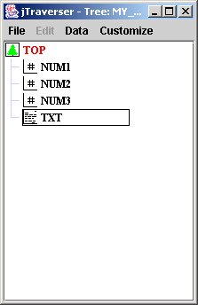
You can see the nodes just created, whose associated icon indicates the usage for that node. When data is inserted in a node, the data access layer of MDSplus checks whether the type of data being inserted matches with the usage for that node.
Using jTraverser, by pressing MB3 button over a node, you can perform the following operations on the node content:
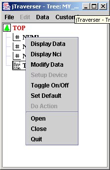
The commands we are interested in, for now, are:
- Display Data: displays the content (if any of the selected node);
- Display NCI: displays accessory node information such as size of contained data, and insertion date;
- Modify Data: modify the content of the node;
When modifying data for node NODE3, jTraverser displays the following dialog:
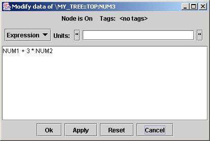
You can type any expression (remember the MDSplus mantra: everything is an expression) which replaces the content of the node.
To experience the check performed on the node usage when inserting data, try to change the content of the node NUM3 to 'This another string' and to save it. You will receive the following error message:
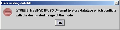
clearly indicating that the usage of that node is not the correct one (it must be an expression returning a numeric value).
Defining a tree structure
Up to now, we have created a flat collection of nodes, possibly containing data. As their name suggests, MDSplus trees allow data to be organized in a hierarchical (tree)structure. Let's do it using TCL, by adding a subtree called SUB1 containing a numeric node SUB_NODE1 and another subtree called SUB2, containing a text node SUB_NODE2.
Open tree my_tree for editing (i.e. adding/removing nodes). The default shot number is -1 (the experiment model)
TCL> edit my_tree
Create a new subtree. Note that the name is preceded by a dot.
TCL> add node .SUB1
Move into SUB1 subtree. Much like the UNIX cd command.
TCL> set def .SUB1
Add empty node SUB_NODE1 to subtree SUB1.
TCL>add node SUB_NODE1/usage=numeric
Create subtree SUB2
TCL> add node .SUB2
Move into SUB2 subtree
TCL>set def .SUB2
Add empty node SUB_NODE2 to subtree SUB2.
TCL> add node SUB_NODE2/usage=text
Write the newly created tree
TCL> write
Close the tree.
TCL> close
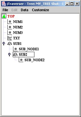
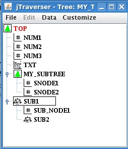
Now, when we open my_tree with jTraverser, and explode subtrees, we get the following image(you can explode/implode subtrees by clicking on the associated handles, or double clicking the subtree):
In the case you are allergic to graphical interfaces, you can nevertheless navigate into the tree structure of the tree using the TCL commands set def <node name> (for moving into a subtree), set def ".-" (for moving one level up) and dir (for showing the content of the current subtree).
Understanding node names
While in a flat list of nodes, the node name is enough to uniquely identify the single data item, in a tree structure, it is necessary to define the whole path. Let's take an example: select the popup item show data in jTraverser over node SUB_NODES2. After enlarging the displayed window we get:
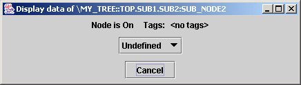
The dialog tells us that the node is undefined (does not contain data yet), and a couple of other information we shall see later. We are now interested in the title of the dialog which shows the path name of node SUB_NODE2. The first part \MY_TREE::TOP indicates the root of tree MY_TREE and the rest of the name is the path from the root to node SUB_NODE2. Observe the dots and the colons: the hierarchy organization in MDSplus trees defines two kinds of nodes for every subtree: members, whose name is preceded by a colon, and children, whose name is preceded by a dot. In this example SUB_NODE2 is a member of node SUB2 which is in turn a child of node SUB1. The MDSplus data organization defines also the concept of default position. Node pathnames can in fact be absolute (i.e. starting from the root) or relative (i.e. starting from the default node), and the default node position is indicated in red in jTraverser and can be changed selecting the popup menu item Set Default (don't worry about it, you will use it very seldom).
Even though MDSplus allows an arbitrary organization of members and children (a member node may have members and/or children), the usual approach is to define members for containing data and children for defining the structure (data cannot never inserted into a child node).
Even in this simple example, it is clear that node pathnames can be very lengthy, increasing also the probability of typing errors. For this reason, MDSplus allows one or mode unique names to be associated with a given node. These identifiers are called tags and are very useful for providing a short and easy name to nodes (usually containing acquired data) which are often referred for data display.
Even though it is possible to define tags in TCL, it is easier to do it with jTraverser. To give tag name MY_SPECIAL_NODE to node \MY_TREE::TOP.SUB1.SUB2:SUB_NODE2 using jTraverser, you need to open experiment my_tree selecting also the edit checkbox in the open dialog. Then you position the mouse over the node, press MB3 button and select the Modify Tags item in the popup menu. You then get the following window:
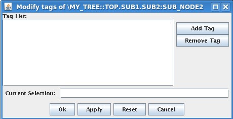
in which you can add/remove the tag name(s) which will be associated with that node. Add MY_SPECIAL_NODE in the list (writing the name in Current Selection Field and then pressing Add Tag button) and press Ok. From now, the tag is associated with that node, and is shown in the data dialog when showing or modifying data.
(Note that in this example, the first time you select the modify data popup item for this node, the node will be shown as undefined, as no data has been added to it in TCL. You can insert new data into it by changing the undefined option into expression and then typing an expression)
Tag names can be used everywhere a node reference is required, e.g. in an expression referring to that node, and the general syntax is:
\<tree name>::<tag name> (e.g. \MY_TREE::MY_SPECIAL_NODE in our example)
When only one tree is open (we shall see in another tutorial that it is possible to open at the same time several trees), the first part (<tree_name>::) may be omitted.
Tag names can be made of up to 24 characters. Node names are instead limited to 12 characters.
The TCL and jTraverser tools
TCL and jTraverser are two equivalent tools, in the sense that both allow the creation and modification of MDSplus trees. It is in fact possible in TCL to navigate into the tree structure using the commands set def and dir. It is even possible to look at data in TCL, but what we see is not exactly what you would expect. Let's try it with the following commands:
TCL>set tree my_tree
Open my_tree experiment model. Note that the command is now set tree, and no more edit. The command edit is required when adding/removing nodes or when changing node names, but is not required for displaying or modifying data associated wit nodes.
TCL>show data NUM3
Want to see data associated with node NUM3. Note that this is a relative path name (colon in front of the name is assumed by default) to the default position which is now the root of the tree. We get the following:
\MY_TREE::TOP:NUM3
DTYPE_FUNCTION : OPC$ADD
DTYPE_NID : \MY_TREE::TOP:NUM1
DTYPE_L : 2
DTYPE_FUNCTION : OPC$MULTIPLY
DTYPE_L : 3
DTYPE_NID : \MY_TREE::TOP:NUM2
DTYPE_L : Array [ 7 ]
Not very clear, isn't it? In fact the show data command displays the internal organization of the information required to specify the expression NUM1 + 3 * NUM2, an information very useful when debugging the system, but surely not easily readable to end users.
On the other side, jTraverser can be used also for changing node names, adding/removing tag names and adding/removing nodes. For these operations you need to select the edit checkbox in the Open dialog. You will note that the popup list in this case is more complete:
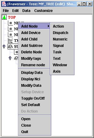
The new commands in which we are interested (the others will be discussed in other tutorials) now are;
- Add Node: add a member node to the selected node (that over which MB3 has been pressed), whose usage is specified by the associated sublist (good occasion for looking at the usages supported by MDSplus - for now we know only Text and Numeric)
- Delete Node: remove the currently selected node;
- Modify Tags: add/remove tag names for this node;
- Rename node: rename the pathname, possibly moving the node to another subtree.(It is also possible to change the name of a node "a la Windows" by slowly clicking twice over the node name, editing the new name, and then hitting <Return> key).
Concluding tip: use TCL for creating and populating a tree the first time. Use jTraverser for looking at it, and for changes in its structure.
Experiment model and pulse files
When you opened tree my_exp with jTraverser you typed -1 as shot number. In MDSplus shot number -1 is used to indicate the experiment model. The experiment model represents the template of the the experiment database, that is the pulse file. A new pulse file will be produced after every experiment, starting from a copy of the experiment model. The experiment model defines the structure of the pulse file, the configuration parameters and the data dependencies, leaving a number of data items empty. There are the data items which will contain data acquired during the experiment, produced by a variety of programs reading data from hardware devices or computing derived data by means of online data analysis.
TCL and jTraverser are typically used on experiment models, singe acquired data will be either accessed by user analysis programs or displayed by data visualization tools like jScope.
Even if not representing the normal use case, TCL can be used also to access and manipulate experiment models. In this case the shot number the edit and set tree commands:
TCL> edit <exp_name>/shot=<shot_number>
or
TCL> set tree <exp_name>/shot=<shot_number>
Recall that edit is used when the structure of the tree is going to be changed (e.g. adding or deleting nodes) requiring issuing a write command at the end. Command set tree is used to open a tree when its structure is not changed, that is when data is read and written, but nodes are neither added nor deleted.
TCL can be used also for creating new pulse files from the template experiment model. The following commands will create a new pulse file with shot number 1 from the experiment model of my_tree
TCL> set tree my_tree
TCL> create pulse 1
TCL> set tree my_tree/shot=1
The last command open the pulse file for further operations. Command create pulse makes a copy of the template experiment model but does not open it.
Merging different trees
In the above example we have created a single tree named my_tree. Looking at the created files (in the directory defined by my_tree_path environment variable) we shall discover that three new files have been created for the experiment model: my_tree_model.characteristics, my_tree_model.datafile, my_tree_model.tree. The pulse files are stored in similar file triplets: my_tree_<shot>.characteristics, my_tree_<shot>.datafile, my_tree_<shot>.tree. These file triplets store data and metadata of my_tree experiment model and pulse files.
Using a single tree may be good for a small experiment, but larger experiments will likely involve different working groups defining and handling their own data. In this case it is possible to let every group define his own experiment model, and then merge all the trees into higher level tree so that, starting from a common root, it is possible to navigate into the whole hierarchy. MDSplus is even more generic and allows for an arbitrary degree of nesting in subtrees. In the following example we shall create a new tree, named my_subtree and then we shall link it to my_tree.
First, we need to define environment variable my_subtree_path to a directory (not necessarily the same as my_tree) with write permission. Then we create a simple tree with two nodes SNODE1 and SNODE2.
TCL> edit my_subtree/new
TCL> add node SNODE1/usage=numeric
TCL> add node SNODE2/usage=numeric
TCL> write
TCL> close
Once tree my_subtree has been created, it can be linked to my_tree. To do this, it suffices adding a new node to my_tree with the same name of the subtree (my_subtree in our example) and usage "subtree":
TCL> edit my_tree
TCL> add node MY_SUBTREE/usage=subtree
TCL> write
TCL> close
At this point linking is done. If we open the experiment model my_tree in jTraverser the new subtree is displayed with the same icon of the tree root (meaning that it is the root of a different tree), and it can be expanded.
It is worth understanding the difference between the node MY_SUBTREE and node SUB1. Both can be expanded when traversing the tree, but the former refers to a different tree hosted in a different triplet of files, while the latter refers to the internal hierarchy of my_tree.
Different subtrees can be linked at different nesting levels. For example subtree my_subtree could be linked in turn to another subtree and so on.
When handling multiple linked trees make sure that the corresponding environment variables <tree_name>_path are defined. If <tree_name>_path for a given subtree is not defined, you will see the icon in the parent tree, but you will not be able to expand it.
As a final remark, you may have noticed that in the former examples always referred to the experiment models. This is the usual approach, and when pulse files are created by the TCL create pulse command, a copy of the template experiment model is recursively performed on all the linked subtrees.
Understanding MDSplus signals
In our current exercise we have dealt with strings, numbers, arrays and expressions. A data type which is very useful in data acquisition is the signal, i.e. an array of data (y axis values) with associated x axis information. Most times, signals refer to some physical signal acquired at a certain frequency for a certain time. In this case the X axis represents the time value of the acquired samples.
MDSplus defines explicitly a data type for signals, and a signal usage for tree nodes. Though signals are usually produced by some data acquisition routine, it is possible to define signals manually. How?? By defining the corresponding expression, of course!
Let's add to my_tree a node called SIGNAL1 containing a sine wave made of 1000 sampled points taken over a period of 1 second.
TCL>edit my_tree
TCL>add node SIGNAL1/usage=signal
TCL>put SIGNAL1 "build_signal(sin(6.28 * [0 .. 999]/1000.),, [0 .. 999]/1000.)"
TCL>write
TCL>close
The TDI expression syntax for defining signals is the following (full reference to TDI expressions is here ):
BUILD_SIGNAL(DATA, RAW, [DIMENSION...])
where:
- DATA is an expression defining the Y values. (sin(6.28 * [0 .. 999]/1000.) in our example)
- RAW is an expression indicating raw data. Often an acquired signal is made of raw data converted then by taking into account parameters such as gain and offset. For the moment we omit its definition (the two commas in the TCL example are not a typing error).
- DIMENSION is an expression returning the array of X axis, usually (but not always) time values. (In our example the expression is [0 .. 999]/1000.)
Now let's check the dimension of the created data item. One may expect that the signal just created will require the bytes necessary to store 1000 float values for the Y value plus 1000 float values for the times. Assuming that 4 bytes are reserved for a floating point number, this yields 8KB. We can inspect the dimension of SIGNAL_1 data item using the popup menu option Display Nci. The window below is shown
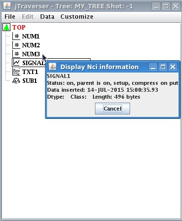 showing that the dimension of the stored item is 496 bytes!!! How can it be?? The reason is that what has been stored in the tree is an expression specifying a sinusoidal signal, NOT the points of the sinusoidal signal itself. However, whenever accessed, such expression will be evaluated on the fly by MDSplus, thus producing the 1000 float values for the Y and X axis, respectively.
This may seems a bit confusing at a first glance, but it allows a very flexible management of raw and derived data in data acquisition. In order to understand it better, let's consider this common use case in data acquisition, where an array of raw samples is read and stored in the tree during data acquisition, together with the associated time values. In addition, converted data can be derived, e.g. by subtracting an offset value and multiplying by a gain factor. If we want to keep in the pulse file both raw and converted data we may think that two different signals need to be stored, thus doubling the required space on disk. This is however not true, since, once raw data are available, only the knowledge of the gain and offset (two scalar values) is required to derive converted data. MDSplus expressions turn out to represent the ideal mean for expressing such dependency in data. We can convince ourselves making the following exercise miming a real data acquisition process (except for the actual dimension of the arrays):
In the first step we prepare an experiment model defining the following nodes:
- RAW_SAMPLES: it will contain the raw samples
- TIMES: it will contain the sample times
- OFFSET: containing the offset value
- GAIN: containing the GAIN value
- SIGNAL2: the complete signal definition that will include both raw data and conversion definition.
These are the TCL commands:
TCL> edit my_tree
TCL> add node RAW_SAMPLES/usage=numeric
TCL> add node TIMES/usage=numeric
TCL> add node OFFSET/usage=numeric
TCL> add node GAIN/usage=numeric
TCL> add node SIGNAL2/usage=signal
Then we define in the experiment model the appropriate expression for SIGNAL2 and the values for GAIN and OFFSET:
TCL> put SIGNAL2 "BUILD_SIGNAL(GAIN*(RAW_SAMPLES - OFFSET),RAW_SAMPLES, TIMES)"
TCL> put OFFSET "0.1"
TCL> put GAIN "2.0"
TCL> write
TCL> close
The first argument pf BUILD_SIGNAL defines converted data, represented by the expression specifying how they are derived from raw samples. The second argument of BUILD_SIGNAL is the reference to raw values and the third one is the reference to the times data item. Recall that data item does not contain actual sample values but only references to other nodes in the tree. Observe also that SIGNAL2 now contains the definition of the signal, but it cannot be evaluated now, since fields RAW_SAMPLES and TIMES referred by the expression do not contain data yet.
In a data acquisition sequence, a pulse file would be created from the experiment model and acquired data written there. We can do the same with the following TCL commands:
Open the experiment model (not in edit mode since we are not changing its structure):
TCL> set tree my_tree
Create pulse file with shot number 1
TCL> create pulse 1
Open pulse file with shot number 1
TCL> set tree my_tree/shot=1
Write raw samples (just ten random values)
TCL> put RAW_SAMPLES "[1,3,5,4,6,2,8,4,9,0]"
Write times (10Hz starting at time 0)
TCL> put TIMES "[0.,0.1,0.2,0.3,0.4,0,5.0.6,0.7,0.8,0.9]"
At this point the pulse file contains the complete definition of both converted and raw signals, even if only the raw data array is actually stored in the pulse file. You may, for example, look at this signal with jScope (see next section).
The evaluation of expression SIGNAL2 yield in this case the array of converted signal values; evaluation of expression RAW_OF(SIGNAL2) yelds the array of raw samples and evaluation of expression DIM_OF(SIGNAL2) yields the array if sample times.
This very simple example highlights once more the different purposes of the experiment model and of the pulse files: the experiment mode will define the structure of the tree, the setup parameters and the data dependencies. The pulse file, initially cloned from the experiment model, will be enriched with acquired data to provide a complete and self-descriptive view of the data dealt with in the experiment.
More on MDSplus expressions
You will have understood that expressions are ubiquitous in MDSplus. Expressions are defined by means of a very rich syntax, called TDI, with tens of possible operators supporting many different data types. Just a few examples of expression:
- 2.3 A floating point number
- 2 + 3.14 A summation evaluated to a floating point number
- 'This is a string' A text string
- 'A string '//'Another string' The concatenation of two strings
- [1,2,5,7] An integer array
- 2. * ([1,2,5,7] + [2,2,2,7]) An (IDL or Matlab like) expression involving scalars and arrays.
- \MY_TREE:NODE1 A reference to a MDSplus tree node
- 2 * (\MY_TREE:NODE1 + 3) An expression involving number and tree nodes
You can do more: it is in fact possible to define variable in TDI. Once defined, they can be later used. For example:
_a = 2 * (\MY_TREE:NODE1 + 3)
                             Assign an expression to variable _a
_b = sqrt(_a)
                             Assign to _b the square root of _a
Remember that TDI variable always begin with an underscore!
You may wonder what are variables useful for. In fact, it makes no sense to use variable in insulated expressions, but expressions can be concatenated to form a TDI function, much like you would do in IDL, MATLAB, or a programming language. Here is an example of a TDI function which returns the sum of all the members in a given array:
fun public vector_sum(in _a)
 {
     _sum = 0;
     for(_i = 0; _i < size(_a); _i++)
         _sum = _sum + _a[_i];
     return(_sum);
 }
Looks like a real program, isn't it? Note that variables (remember the underscore!!) are not declared, and can contain any type of data.
You save this function in a text file called vector_sum.fun and you put it in a subdirectory of MDSPLUS_DIR/tdi, where MDSPLUS_DIR is the root of the MDSplus distribution of your system.
After copying it in the right place, you can use without any compilation. Here is an example of usage:
 _arr = [1,2,4,5];
 _sum = vector_sum(_arr);
 write(*, 'The sum of the elements of ', _arr, ' is ', _sum);
 _sum2 = 2 * vector_sum(_arr);
As everybody who wrote a program knows, it is possible to make syntax errors when writing TDI expressions and programs. As there is no compilation, the errors arise when that expression is evaluated. The error message is often not very clear (just to be polite  ), so correcting errors when writing TDI functions my be very frustrating. In this case the tdic tool for debugging MDSplus expressions can be very useful, and allows to spare quite a lot of debugging time. ), so correcting errors when writing TDI functions my be very frustrating. In this case the tdic tool for debugging MDSplus expressions can be very useful, and allows to spare quite a lot of debugging time.
When launched with the command tdic, the tool provides the evaluation on the fly of the expression passed in the command line (preceded buy the TDI> cursor). tdic looks similar to a online calculator:
 TDI> 2+3
 5
In this case the expression to be evaluated is just the sum of two integer numbers. We can use this tool to evaluate the content of the tree node, however it is necessary to open first the tree, using the pre-defined expression treeopen(<exp_name>,<shot>):
TDI> treeopen("my_tree",1)
265388041
TDI> NUM1
2
TDI> NUM2
[1,2,3,4,5,6,7]
TDI> NUM3
[5,8,11,14,17,20,23]
The strange number reported by treeopen() is the return status of the the tdi pre-defined function treeopen(). Recall: tdic simply takes the typed line and evaluates it. Recall that the expression stored in NUM3 was NUM1+3*NUM2. When using tdic to look at the signals stored in the previous example in pulse file with shot number 1 we get:
TDI> treeopen("my_tree",1)
265388041
TDI> SIGNAL2
Build_Signal(GAIN * (RAW_SAMPLES - OFFSET), RAW_SAMPLES, TIMES)
TDI> data(SIGNAL2)
[1.8,5.8,11.8,13.8,15.8,7.8,9.8,11.8,13.8,9.8,11.8]
TDI> data(RAW_OF(SIGNAL2))
[1,3,6,7,8,4,5,6,7,5,6]
TDI> data(DIM_OF(SIGNAL2))
[1,2,3,4,5,6,7,8,9,10]
Things are now a bit more tricky...when evaluating expression SIGNAL2 (after opening the pulse file we used to put raw data and times in the previous example) we may expect to get the signal samples, but we got a more complex thing. In fact the signal type is one of the types supported by MDSplus and is returned by evaluating expression SIGNAL2, that is, by reading the content of node SIGNAL2. It is however possible to force a further degree of evaluation using keyword data(). In this case the result will be either a scalar or array. data(SIGNAL2) will yield the converted samples of the signal. Similarly the actual raw samples and the associated times arrays can be evaluated.
Python integration in MDSplus expressions
We shall see in the next sections that MDSplus is deeply integrated in python and all the MDSplus functionality is available when programming in python. The converse is also true, that is, it is possible to define python functions and use them in MDSplus expression.
We have seen in the previous section how a new function written in TDI can be defined so that it can be included in MDSplus expressions. We shall now do the same with a sample function my_python_sum written in python, making the sum of two numbers (scalar or arrays).
def my_python_sum(a,b):
    return a+b
The python code must be saved in a file with the same name of the function (my_python_sum.py in this case) and in the directory referred by env variable MDS_PATH. This is the only required action to let MDSplus handle the python function in expressions.
We can exercise this python function in expression evaluation using tdic:
TDI> treeopen("my_tree",-1)
265388041
TDI> NUM2
[1,2,3,4,5,6,7]
TDI> my_python_sum(2,3)
5
TDI> my_python_sum(2,[1,2,3])
[3,4,5]
TDI> my_python_sum(2,NUM2)
[3,4,5,6,7,8,9]
We can do even more, that is, we can store in a MDSplus tree an expression which includes python function calls. Let's do it in my_tree:
TCL> set tree my_tree
TCL> put NUM3 "my_python_sum(NUM1, NUM2)"
And then let's evaluate NUM3 in tdic:
TDI> treeopen("my_tree",-1)
265388041
TDI> NUM1
2
TDI> NUM2
[1,2,3,4,5,6,7]
TDI> NUM3
[3,4,5,6,7,8,9]
Recall that NUM3 does not contain the array itself, but the specification of a MDSplus expression implying the activation of the python function my_python_sum(). When evaluated, thw function is executed on the fly yielding the expected result.
What next?
We have now learnt how to build and populate a MDSplus tree and some basic concepts about MDSplus data. We know also how references into the tree are specified and we know that it is possible to use expressions for a flexible definition of data.
We are now ready to go further, and to access data contained in the tree. The next tutorial will show you how to export MDSplus trees over the network, and how to access data from programs and from jScope, the MDSplus tool for waveform display.
| 


