From MdsWiki
| Revision as of 10:37, 25 June 2015 (edit) Manduchi (Talk | contribs) (→A quick tour over MDSplus) ← Previous diff |
Revision as of 12:47, 25 June 2015 (edit) Manduchi (Talk | contribs) (→Tutorial 1: MDSPlus Experiment Model and pulse file and their interfaces) Next diff → |
||
| Line 24: | Line 24: | ||
| describing a clock starting at ''StartTime'', ending at ''EndTime'' and with period ''Period''. Here StartTime, EndTime and Period are not directly represented by numbers, but they refer to other data items in the TIMING subtrees, i.e. TRIGGER, DURATION and FREQUENCY. This particular expression defines a clock which starts at the time specified in TRIGGER item, lasts the time specified in DURATION item and whose period is the reciprocal of the frequency value specified in FREQUENCY item.<br /> | describing a clock starting at ''StartTime'', ending at ''EndTime'' and with period ''Period''. Here StartTime, EndTime and Period are not directly represented by numbers, but they refer to other data items in the TIMING subtrees, i.e. TRIGGER, DURATION and FREQUENCY. This particular expression defines a clock which starts at the time specified in TRIGGER item, lasts the time specified in DURATION item and whose period is the reciprocal of the frequency value specified in FREQUENCY item.<br /> | ||
| Let's now expand sibtree RAW: a sequence of nodes named SIG_1 to SIG_16 is shown, with a different associated icon. That icon means that those nodes are designed to containg a ''Signal'' data type. Without entering into details for now, the Signal data types defines an array of values, that is, the samples of the acquiered signal, and an array of times, that is, the time of every sample. Users are normally not concerned with the details of the Signal representation because signals object are managed by MDSplus providing the samples and the times when requested. <br /> | Let's now expand sibtree RAW: a sequence of nodes named SIG_1 to SIG_16 is shown, with a different associated icon. That icon means that those nodes are designed to containg a ''Signal'' data type. Without entering into details for now, the Signal data types defines an array of values, that is, the samples of the acquiered signal, and an array of times, that is, the time of every sample. Users are normally not concerned with the details of the Signal representation because signals object are managed by MDSplus providing the samples and the times when requested. <br /> | ||
| - | Try now to look at the content of SIG_1 node with the "Display Data" popup option. There is no data! This is however not a surprise if you recall the meaning of the Expeirment Model (this jTraverser window is open at shot -1). Signals are typically acquired during the experiment and therefore they will be eventually available in the Pulse File. In our example they have eben put in the RAW subtree, suggesting that thise signals will contain raw samples. Normally the actual values of a signal are the result of some sort of processing from the raw samples. For example, ADC data tyoically require calibration, that is, adding and offset and multiplying them for a gain. In MDSplus this sort of processing becomes natural thanks to expressions. Have a look at the signals defined in the CALIBRATED subtree, which are intended, in this example, to represent the calibrated version of the the signals in RAW subtree. In most data acquisition systems, calibrated data are stored as an array which si different from the raw data. In MDSplus you can avoid this, just defining the expression which converts raw ata into calibrated ones. Have a look at the expression defined fir CALIBRATED:SIG_1<br /> | + | Try now to look at the content of SIG_1 node with the "Display Data" popup option. There is no data! This is however not a surprise if you recall the meaning of the Experiment Model (this jTraverser window is open at shot -1). Signals are typically acquired during the experiment and therefore they will be eventually available in the Pulse File. In our example they have eben put in the RAW subtree, suggesting that thise signals will contain raw samples. Normally the actual values of a signal are the result of some sort of processing from the raw samples. For example, ADC data tyoically require calibration, that is, adding and offset and multiplying them for a gain. In MDSplus this sort of processing becomes natural thanks to expressions. Have a look at the signals defined in the CALIBRATED subtree, which are intended, in this example, to represent the calibrated version of the the signals in RAW subtree. In most data acquisition systems, calibrated data are stored as an array which si different from the raw data. In MDSplus you can avoid this, just defining the expression which converts raw ata into calibrated ones. Have a look at the expression defined fir CALIBRATED:SIG_1<br /> |
| [[Image:ExampleTree3.jpg]] <br /> | [[Image:ExampleTree3.jpg]] <br /> | ||
| - | The shown expression specifies that the raw signal in node RAW:SIG_1 is multiplied by 10./4096 (this is the conversion for a +- 5V, 12 bits ADC), that the offset value specified in node PARAMETERS:OFFSET is subtracted and the result miltiplied by the value stored in node PARATEMETS:GAIN. Observe that what is stored in node CONVERTED:SIG_1 is just the expression definition, not the actual value array. When CONVERTED:SIG_1 is evaluated, e.g. when it is read by a user program, MDSplus performs an evalation on the fly, returning the actual array of converted values for that signal. Observe also that, while RAW:SIG_1 node is empty, CONVERTED:SIG_1 is not empty and contains already the expression definition in the experiment model. If evaluated before data are written in RAW:SIG_1 MDSplus will raise an error stating that the expression cannot be evaluated. After raw data have been written, the evaluation of CONVERTED:SIG_1 will yeld the correct result. | + | The shown expression specifies that the raw signal in node RAW:SIG_1 is multiplied by 10./4096 (this is the conversion for a +- 5V, 12 bits ADC), that the offset value specified in node PARAMETERS:OFFSET is subtracted and the result miltiplied by the value stored in node PARATEMETS:GAIN. Observe that what is stored in node CONVERTED:SIG_1 is just the expression definition, not the actual value array. When CONVERTED:SIG_1 is evaluated, e.g. when it is read by a user program, MDSplus performs an evalation on the fly, returning the actual array of converted values for that signal. Observe also that, while RAW:SIG_1 node is empty, CONVERTED:SIG_1 is not empty and contains already the expression definition in the experiment model. If evaluated before data are written in RAW:SIG_1 MDSplus will raise an error stating that the expression cannot be evaluated. After raw data have been written, the evaluation of CONVERTED:SIG_1 will yield the correct result.<br /><br /> |
| + | The few examples presented so far have illustrated the flexibility on data representation offered by MDSplus. However data dealt with in an experiment can be even richer. Consider for example the required configuration of the hardware devices involved in data acquisition: configuration parameters will be stored in the experiment model in order to properly configure the expeirment. Since a set of data items will specify the configuration of a given device, and several instances of the same device type will be likely defined in the experment, it is useful to provide a sort of "encapsulation" for sets of related data items (such as the configuration parameters of a given device instance). MDSplus allows this encapsulation process by allowing users define a set of device classes, which are then recognized by the system and handled accordligly. Let's expand the DEVICES subtree in our experiment model. Nodes ADC_1 to ADC_4 are shown with a new icon, clocking on any of these nodes we'll discover that it is not a data item, but the root node of a subtree, as shown below.<br /> | ||
| + | |||
| + | If we expand any node we shall discover that all them have the ''same'' subtree structure. ADC_1 to ADC_4 are indeed instances of the same device type. If an instance of a different device type were present here, its subtree will likely have a different structure. We may browse the content of devices exactly at the same way as browsing the rest of the Experiment tree, but MDSplus can recognize devices and present a more specialized interface, activated via the Setup Device popup menu item. Below is the interface for the device class used in this tutorial, basically exposing the content of the underlying subtree, but in a more user friendly organization. <br /> | ||
| + | |||
| + | A set of MDSplus devices is already available in the MDSPlus distribution, but new devices can be defined by users thus providing a personalization of MDSplus for the specific system. Section xx explains how developing new devices in MDSplus. | ||
Revision as of 12:47, 25 June 2015
A quick tour over MDSplus concepts
In this section we'll discover the basic concepts of MDSplus through a set of working examples. We shall skip here most details, covered by the following sections of the tutorial, in order to concentrate on the main concepts.
To run the examples we need first a running installation of MDSplus. The reference system for the presented examples is Linux, although MDSplus can run also on Windows and MacOS. The preparatory steps for this overview are:
- Installation of MDSplus. MDSplus can be installedon several platform and for Linux platforms you can also download the sources and then build the system. Refer to Download Page to install MDSplus on your system.
- Installation of the running examples. The examples are available on GitHub and you can donwload them with the git command
git clone https://github.com/MDSplus/MDSplusTutorial.git
Once the examples have been downloaded from git, move to MDSplusTutorial directory:
cd MDSplusTutorial
and we are ready to start. There are two examples, activated by commands start_tutorial_1 and start_tutorial_2, respectively.
Tutorial 1: MDSPlus Experiment Model and pulse file and their interfaces
Let's start with the first one and type
./start_tutorial_1
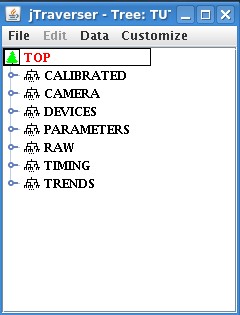
You will see the activation several graphical intefaces and a X Terminal. Let's concentrate on the following window showing a hierarchical structure.

That tree structure displays the hierarchical structure of an Experiment Model, that is the database containing all the data dealt with by the system. Data are stored in database in a hierachical organization, reflecting the normal way information is arranged in scientific applications. A MDSplus database takes two names, that refer to two different stages of the experimental sequence: the Experiment Model and the Pulse file. Consider the execution of a set of measurements that we shall call "experiment". Typically such execution produces data that need to be collected to be analyzed. Experimental data alone however may be not enough, because it is also necessary to know the configuration of all the involved devices in order to give a meaning top thje acquired values. A subset of experimental data will be therefore be represented by configuration information and will be defined before the experiment. This is the typical content of the MDSplus Experiment Model, that is a template of the full database containing configuration data. Observe that typically what happens during an experiment will depend on the actual configuration, i.e. on the data defined in the experiment model. The experiment model is then filled with expeirmental data, eventually producing a database containg the complete description of one experiment, thai is, the Pulse File. In a typical sequece of repeated experiements, the current Experiment Model is copied into a new (incomplete) pulse file just before the experiment sequence. The jTraverser application provides a graphical browser to experiment models, showing the underlying structure and the contained data.
A name and a number are associated with Pulse Files. The number is normally called shot number and refers to the instance number of the pulse file. As an experiment is typically repeated several times, a sequence of pulse files with different shot numbers will be produced as well. The conventional shot number for the Experiment Model is -1.
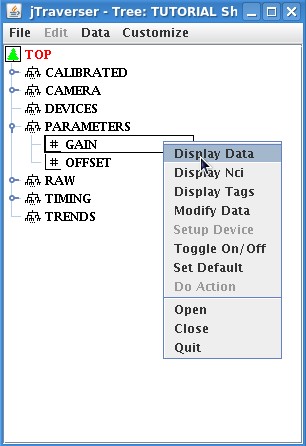
A fairly complete set of data types are supportwed in MDSplus, reflecting te variety of data types dealt with in experiments. Let's have a look at the simplest types and expand PARAMETERS node.

The PARAMETER node has two children nodes: GAIN and OFFSET containing scalar data. You can look at their content via the popup menu as shown in the figure.
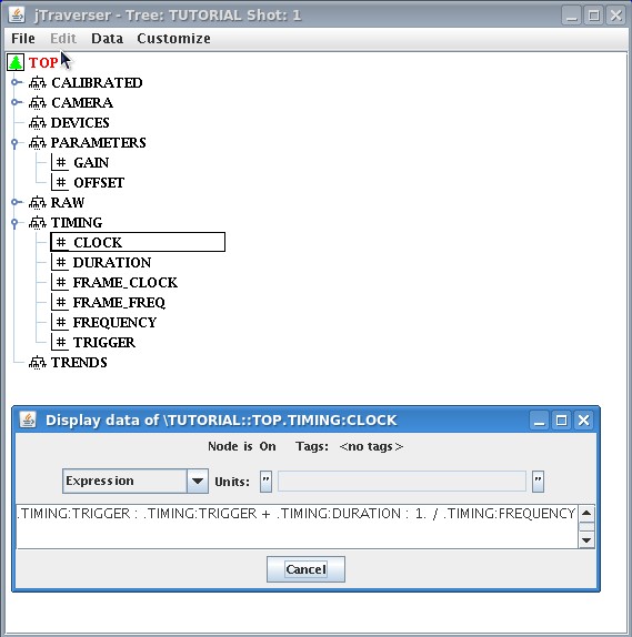
More complex data types can be defined, too. The list of data types supported in MDSplus is very long. More in general, any data item can be represented by an expression that is a combination of operators, numbers and refereces to other data items in the pulse file. Take for example the content of node TIMING.CLOCK shown below

This data item describes a timebase and when evaluated (expressions are always evaluated on the fly by MDSplus when read) it returns the array of times corresponding to the specified clock. Its definition is of the form
<StartTime>:<EndTime>:<Period>
describing a clock starting at StartTime, ending at EndTime and with period Period. Here StartTime, EndTime and Period are not directly represented by numbers, but they refer to other data items in the TIMING subtrees, i.e. TRIGGER, DURATION and FREQUENCY. This particular expression defines a clock which starts at the time specified in TRIGGER item, lasts the time specified in DURATION item and whose period is the reciprocal of the frequency value specified in FREQUENCY item.
Let's now expand sibtree RAW: a sequence of nodes named SIG_1 to SIG_16 is shown, with a different associated icon. That icon means that those nodes are designed to containg a Signal data type. Without entering into details for now, the Signal data types defines an array of values, that is, the samples of the acquiered signal, and an array of times, that is, the time of every sample. Users are normally not concerned with the details of the Signal representation because signals object are managed by MDSplus providing the samples and the times when requested.
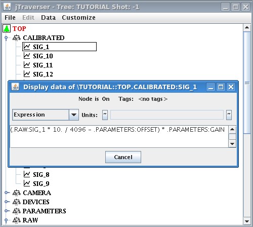
Try now to look at the content of SIG_1 node with the "Display Data" popup option. There is no data! This is however not a surprise if you recall the meaning of the Experiment Model (this jTraverser window is open at shot -1). Signals are typically acquired during the experiment and therefore they will be eventually available in the Pulse File. In our example they have eben put in the RAW subtree, suggesting that thise signals will contain raw samples. Normally the actual values of a signal are the result of some sort of processing from the raw samples. For example, ADC data tyoically require calibration, that is, adding and offset and multiplying them for a gain. In MDSplus this sort of processing becomes natural thanks to expressions. Have a look at the signals defined in the CALIBRATED subtree, which are intended, in this example, to represent the calibrated version of the the signals in RAW subtree. In most data acquisition systems, calibrated data are stored as an array which si different from the raw data. In MDSplus you can avoid this, just defining the expression which converts raw ata into calibrated ones. Have a look at the expression defined fir CALIBRATED:SIG_1

The shown expression specifies that the raw signal in node RAW:SIG_1 is multiplied by 10./4096 (this is the conversion for a +- 5V, 12 bits ADC), that the offset value specified in node PARAMETERS:OFFSET is subtracted and the result miltiplied by the value stored in node PARATEMETS:GAIN. Observe that what is stored in node CONVERTED:SIG_1 is just the expression definition, not the actual value array. When CONVERTED:SIG_1 is evaluated, e.g. when it is read by a user program, MDSplus performs an evalation on the fly, returning the actual array of converted values for that signal. Observe also that, while RAW:SIG_1 node is empty, CONVERTED:SIG_1 is not empty and contains already the expression definition in the experiment model. If evaluated before data are written in RAW:SIG_1 MDSplus will raise an error stating that the expression cannot be evaluated. After raw data have been written, the evaluation of CONVERTED:SIG_1 will yield the correct result.
The few examples presented so far have illustrated the flexibility on data representation offered by MDSplus. However data dealt with in an experiment can be even richer. Consider for example the required configuration of the hardware devices involved in data acquisition: configuration parameters will be stored in the experiment model in order to properly configure the expeirment. Since a set of data items will specify the configuration of a given device, and several instances of the same device type will be likely defined in the experment, it is useful to provide a sort of "encapsulation" for sets of related data items (such as the configuration parameters of a given device instance). MDSplus allows this encapsulation process by allowing users define a set of device classes, which are then recognized by the system and handled accordligly. Let's expand the DEVICES subtree in our experiment model. Nodes ADC_1 to ADC_4 are shown with a new icon, clocking on any of these nodes we'll discover that it is not a data item, but the root node of a subtree, as shown below.
If we expand any node we shall discover that all them have the same subtree structure. ADC_1 to ADC_4 are indeed instances of the same device type. If an instance of a different device type were present here, its subtree will likely have a different structure. We may browse the content of devices exactly at the same way as browsing the rest of the Experiment tree, but MDSplus can recognize devices and present a more specialized interface, activated via the Setup Device popup menu item. Below is the interface for the device class used in this tutorial, basically exposing the content of the underlying subtree, but in a more user friendly organization.
A set of MDSplus devices is already available in the MDSPlus distribution, but new devices can be defined by users thus providing a personalization of MDSplus for the specific system. Section xx explains how developing new devices in MDSplus.